Multi-run simulations in LWFBrook90R
Source:vignettes/LWFBrook90R-3-Multiruns.Rmd
LWFBrook90R-3-Multiruns.RmdIntroduction
With ‘LWFBrook90R’, parallelized multi-run simulations can be
performed conveniently, extending the basic single-run applications
using the function run_LWFB90() described in the
introductory vignette. Two different multi-run functions exist for two
different problems:
- Perform Monte-Carlo simulations with single parameters set up for variation, and
- simulations over multiple locations, parameter sets, or climate scenarios.
For the first case, the function run_multi_LWFB90() is
available. The second problem can be tackled using the function
run_multisite_LWFB90(), which is described in detail in the
vignette ‘Multi-Site
simulations’.
Both functions are wrapper functions for run_LWFB90()
and allow for parallel processing of tasks, using a specified number of
CPUs to speed up the execution of a multi-run simulation. They return
lists containing the individual single run simulation results, as they
are returned by run_LWFB90(). These result-lists can become
very large if many simulations are performed, and the selected output
comprises daily data sets and especially the individual soil layers’
daily soil moisture states. Huge amounts of data produced can overload
the memory, this vignette therefore starts with a data management
section on how to make best use of the output_fun-argument
of run_LWFB90() to reduce the amount of data returned.
Data management (i): output_fun-argument
To minimize memory allocation, it is recommended to reduce the
selected output to a minimum and make use of the
output_fun-argument of run_LWFB90(). With this
argument, it is possible to pass custom functions to
run_LWFB90(), which directly perform on the simulation
output list object. With rtrn_output = FALSE, the original
simulation output (output, layer_output) then
can be discarded, and only the results from the
output_fun-argument are returned. This can be very useful
for model calibration or sensitivity analyses tasks comprising ten
thousands of simulations in a Monte-Carlo setting. With this magnitude,
memory allocation is critical, and only a relatively small output can be
returned for each individual simulation (e.g., a measure of agreement
between simulated and observed values). Similarly, it is possible to
define functions for custom output aggregation, or to redirect the
simulation output to a file or database, as we will see later.
To demonstrate the usage of the output_fun-argument, we
perform a Monte-Carlo simulation using the function
run_multi_LWFB90(), and define a function that returns
annual mean soil water storage and transpiration during the growing
season. In a first step, the function integrates depth-specific soil
moisture to soil water storage down to specified soil layer
(tolayer, passed via ... to
output_fun), and in a second step calculates mean soil
water storage over the growing season, along with the sum of
transpiration. The growing season thereby is defined by the input
parameters budburstdoy and leaffalldoy.
output_function <- function(x, tolayer) {
  # aggregate SWAT
  swat_tran <- x$layer_output[which(nl <= tolayer),
                              list(swat = sum(swati)),
                              by  = list(yr, doy)]
  #add transpiration from EVAPDAY.ASC
  swat_tran$tran <- x$output$tran

  # get beginning and end of growing season from input parameters
  vpstart <- x$model_input$param_b90$budburstdoy
  vpend <- x$model_input$param_b90$leaffalldoy
  swat_tran <- merge(swat_tran,
                     data.frame(yr = unique(swat_tran$yr),
                                vpstart, vpend), by = "yr")
  # mean swat and tran sum
  swat_tran[doy >= vpstart & doy <= vpend,
            list(swat_vp_mean = mean(swat), tran_vp_sum = sum(tran)), by = yr]
}
To test our custom output function we run a single-run simulation
data("slb1_meteo")
data("slb1_soil")
soil <- cbind(slb1_soil, hydpar_wessolek_tab(texture = slb1_soil$texture))
b90res <- run_LWFB90(options_b90 = set_optionsLWFB90(),
                     param_b90 = set_paramLWFB90(),
                     climate = slb1_meteo,
                     soil = soil)
and apply the function to the return, to see that our custom output function works:
output_function(b90res, tolayer = 15)
#> Key: <yr>
#>       yr swat_vp_mean tran_vp_sum
#>    <num>        <num>       <num>
#> 1:  2002     290.1533    202.9172
#> 2:  2003     226.4391    305.4688
Multi-run simulations with run_multi_LWFB90()
As mentioned, run_multi_LWFB90() is a wrapper for
run_LWFB90(). run_multi_LWFB90() takes a
data.frame paramvar containing variable parameter values in
columns and their realizations in rows. For each row in
paramvar, the respective parameter values in
param_b90 are replaced by name, and
run_LWFB90() is called. Further arguments to
run_LWFB90() have to be specified and are passed on.
For the multi-run simulation, we set up two parameters for variation,
the maximum leaf area index (maxlai) and the maximum leaf
conductance (glmax). We define a data.frame with two
columns, containing 50 random uniform realizations of the two
parameters:
set.seed(2021)
N=50
paramvar <- data.frame(maxlai = runif(N, 4,7),
                       glmax = runif(N,0.003, 0.01))
Now we can run the simulation. We suppress the selected simulation
result objects and model input from being returned, and only return the
values from our output_fun defined above. We pass
tolayer = 15 so that soil water storage is integrated down
to the 15th soil layer, corresponding to 0-100 cm soil depth. Note that
the param_b90 object (and thus parameters
budburstdoy and leaffalldoy) is available to
our output_fun, although it is not included in the return
(rtrn_input = FALSE).
mrun_res <- run_multi_LWFB90(paramvar = paramvar,
                             param_b90 = set_paramLWFB90(),
                             cores = 2, # arguments below are passed to run_LWFB90()
                             options_b90 = set_optionsLWFB90(),
                             climate = slb1_meteo,
                             soil = soil,
                             rtrn_input = FALSE, rtrn_output = FALSE,
                             output_fun = output_function,
                             tolayer = 15) # argument to output_fun
The result is a list of the individual single-run results, from which
we can easily extract the results of our output function and
rbindlist() them together in a data.table:
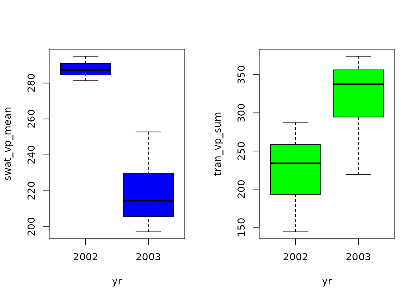
Now we can display the results of the 50 simulations using boxplots:

Growing season soil water storage and transpiration of 50 simulations, with random variation of parameters ‘maxlai’ and ‘glmax’
We ran 50 simulations, all with the same climate, soil, and
parameters except for maxlai and glmax, that
where varied randomly. In the next vignette ‘Multi-Site simulations’,
we will learn how to make use of multiple climate, soil, and parameter
sets using the function run_multisite_LWFB90(), to simulate
a set of different sites.