Introduction
LWF-BROOK90 (Hammel and Kennel 2001) is a soil vegetation atmosphere transport (SVAT) model to calculate daily evaporation (transpiration, interception, and soil evaporation) and soil water fluxes, along with soil water contents and soil water tension of a soil profile covered with vegetation. It is an upgraded version of the original BROOK90 model (Federer, Vörösmarty, and Fekete 2003; Federer 2002), featuring additional parameterizations of the soil water retention and conductivity functions (Mualem 1976; Genuchten 1980), and the option to take interannual variation of aboveground vegetation characteristics into account.
The package core function run_LWFB90() runs the
LWF-Brook90 by:
- creating model input objects from climate driving data, model control options and parameters,
- executing the model code,
- returning the model output.
The model control options thereby let you select different functions for defining aboveground stand dynamics, phenology, and root length density depth distributions. Additionally, a set of pedotransfer functions is provided to derive hydraulic parameters from soil physical properties.
In this vignette, we will use meteorological and soil data from the longterm monitoring beech forest site SLB1 in the Solling mountains, Germany, which are available after loading the package.
To reproduce the examples, load ‘LWFBrook90R’ and the ‘data.table’ package:
Basic usage
Input Objects
As a first step, we need to set up the input objects for the central
function runLWFB90(). Aside from meteorological and soil
data, we need to define the model control options and model parameter
objects. The model options contain basic information about the
simulation and which sub-models to use (e.g. the start and end dates of
the simulation, the precipitation interval, the phenology model, root
length density depth distribution function, etc). The model parameter
object contains about 100 parameters, of which most are required to run
the model, but some only take effect if certain model control options
are selected (see vignette Model control options and
parameters). Two functions are available that can be used to
generate default lists of model options and parameters:
options_b90 <- set_optionsLWFB90()
param_b90 <- set_paramLWFB90()
The created objects can be easily manipulated by reference, or simply
by assigning values to the option and parameter names directly in the
function calls. To look up the meanings of the various options and
parameters see ?set_optionsLWFB90 and
?set_paramLWFB90. The meaning and context of most input
parameters (and output variables) can also be looked up in the
documentation of the original BROOK90 model version on Tony Federer’s
webpages, which is always a recommended source of information when
working with any BROOK90 version.
To run LWF-BROOK90 for the Solling beech site, we need to prepare the
soil data for the model. The data.frame slb1_soil contains
soil physical data of the soil horizons, but not yet the hydraulic
parameters that LWF-BROOK90 requires. Fortunately, ‘LWFBrook90R’ comes
with a set of pedotransfer functions to derive the Mualem/van Genuchten
(MvG) parameters of the soil water retention and hydraulic conductivity
functions. Here we use texture tabulated values from Wessolek, Renger
& Kaupenjohann (2009) and create a
data.frame containing the required MvG-parameters along with the soil
physical data:
soil <- cbind(slb1_soil, hydpar_wessolek_tab(texture = slb1_soil$texture))Single-run simulation
Now we load meteorological dat, and then we are ready to perform a
single-run simulation using the function run_LWFB90():
data("slb1_meteo")
b90res <- run_LWFB90(options_b90 = options_b90,
                     param_b90 = param_b90,
                     climate = slb1_meteo,
                     soil = soil)
run_LWFB90() thereby derives the daily stand properties
(lai, sai, height,
densef, age) and root distribution from
parameters, and passes climate, vegetation properties and parameters to
the Fortran dynamic library. After the simulation has finished, a list
with model output (output, layer_output) is
returned, along with the model input (options_b90,
param_b90 and derived daily vegetation properties
standprop_daily):
str(b90res, max.level = 1)
#> List of 5
#>  $ simulation_duration: 'difftime' num 4.07710194587708
#>   ..- attr(*, "units")= chr "secs"
#>  $ finishing_time     : POSIXct[1:1], format: "2022-06-10 08:05:46"
#>  $ model_input        :List of 3
#>  $ output             :Classes 'data.table' and 'data.frame':    730 obs. of  47 variables:
#>   ..- attr(*, ".internal.selfref")=<externalptr>
#>  $ layer_output       :Classes 'data.table' and 'data.frame':    15330 obs. of  15 variables:
#>   ..- attr(*, ".internal.selfref")=<externalptr>
The list entry output contains calendar variables (‘yr’,
‘mo’, ‘da’, ‘doy’), daily actual evaporation fluxes (‘evap’, ‘tran’,
‘irvp’, ‘isvp’, ‘slvp’, ‘snvp’), potential evaporation and transpiration
fluxes (‘pint’, ‘pslvp’, ‘ptran’), soil water flux (‘flow’, ‘vrfln’) and
state variables (‘swat’, ‘awat’, ‘relawat’). For a detailed description
of all output variables refer to the help pages
(?run_LWFB90).
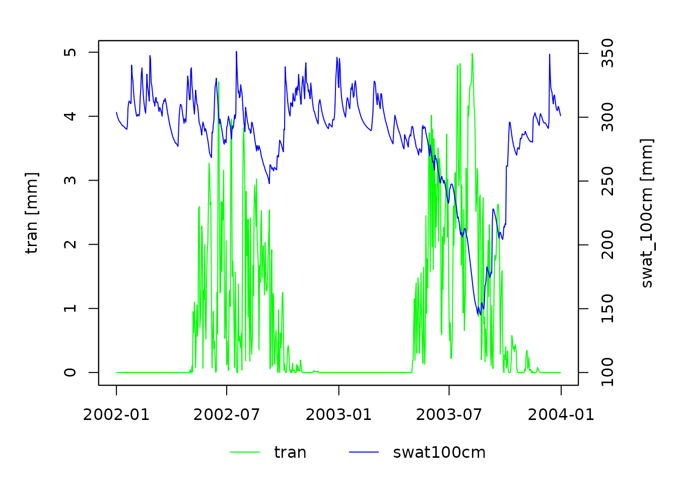
To plot the data, it is convenient to derive a Date
object from the calendar variables. We use data.table syntax here:
A second result set (list item layer_output) contains
daily soil moisture state variables and belowground water fluxes of the
individual soil layers. We want to plot absolute soil water storage
(‘swati’) down to a soil depth of 100 cm, so we need to integrate
b90res$layer_output$swati over the 15 uppermost soil
layers:
b90res$layer_output[, dates := as.Date(paste(yr, mo, da, sep = "-"))]
swat100cm <- b90res$layer_output[which(nl <= 15), list(swat100cm = sum(swati)),
                                by  = dates]
Now we can plot soil water storage and transpiration:

Simulation results for sample data